Corncob can get a surprising amount of mileage out of a grey circle. Put one above a brown polygon and it is a ground crew member’s head. Put several below a vehicle and they are wheels. Make one enormous, change its colour every frame, and it is alien technology.
The rest of the picture is similarly economical. The landscape is mostly a division between sky and ground. An aircraft is a short sequence of flat shapes. Hidden surfaces disappear because somebody arranged for another shape to be drawn over them. Sometimes they don’t disappear, which is how we ended up investigating a tower door visible through the back of its own building.
There is plenty to learn from following those decisions down to the pixels. We’ll use normal retail Corncob 3D 3.42 as our reference, with the preserved assembly source to explain the machinery. Our reconstruction and tests against the original executable help check the interpretation. Source-only experiments and Redux changes are identified separately.
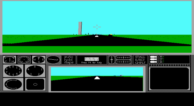
A frame, before the details
Imagine a flight over the airfield. The engine needs the observer’s position and attitude, the nearby objects, their current appearances, and a place in video memory to draw. Most of the scene follows this route:
- Prepare the view.Choose the front and rear windows, update the camera transform and repair their borders.
- Lay down the background.Draw the horizon’s sky and ground fills, motion-cue dots, stars and sun as applicable.
- Visit the objects.Work from the active world data and distance-ordered object list. Ground-level runway pieces get special treatment.
- Run a model’s drawing list.Choose detail and one of eight viewing directions, transform its coordinates and issue its primitives.
- Turn geometry into pixels.Clip, project, walk edges and write masked spans, lines, points or discs.
- Finish and show the page.Update cockpit marks and instruments, then change which video-memory page the display scans.
This is a guide to the drawing work, not six neatly separated modules in the original program. Object timers, collision checks, walking height and drawing share parts of the traversal. The source is quite happy to ask whether we have crashed while working its way through things to draw.
The decisive omission is a depth buffer. There is no second image storing the distance to whatever owns each pixel. A later opaque write replaces an earlier one. Corncob therefore has to arrange visibility before, and through, the drawing order.
Four kinds of mark
The flight executable contains 61 object templates. These provide model pointers, distance limits and other properties. A model then points to small primitive records. Its drawing vocabulary is compact:
| Code | Primitive | What it supplies |
|---|---|---|
| 0 | Nothing | A deliberately empty command slot. |
| 2 | Connected lines | Lists of coloured polylines with consecutive XYZ vertices. |
| 4 | Points | XYZ positions with individual colours. |
| 6 | Discs | XYZ centres, diameters and colours. |
| 8 | Filled polygon | A colour and an ordered ring of XYZ vertices. |
There are no texture coordinates in these records, and no normal vectors for a lighting calculation. A painted marking is more geometry, or a line drawn over geometry. A round object can be a disc. The model’s different flat colours provide much of what we read as shading.

The ground crew demonstrate the whole approach particularly well. Their bodies are flat polygons; their heads and eyes are discs; the mouth is linework. We initially read the disc size as a radius and gave everybody a swollen head. The original code uses a diameter, halving it only when it comes to finding the edges on screen. The same mistake made vehicle wheels enormous.
Animation often means changing these inputs. The crew’s raised finger is a model swap. A dish turns by changing its orientation. Fire moves stored particle centres and sizes. Forcefields alter geometry, while other effects change colour variables. There is no need to invent a skeletal animation system to explain any of that.
Explore the recovered models →
A large world in small integers
The world files divide their contents into an 8 × 8 grid. Each tile is 2,097,152 centimetres across: about 20.97 km. The whole storage grid spans about 167.77 km on either horizontal axis. That describes the addressable layout, not a promise of populated scenery across the entire square.
Objects have 32-bit world positions in centimetres. Model vertices use signed 16-bit coordinates, with two centimetres per model unit. The renderer has to bring these scales together without letting an enormous world position spill into a tiny local coordinate.
First subtract the observer’s position from the object’s position. The absolute address of the airfield is no longer important; only its displacement from us matters. Corncob then classifies that displacement by the largest absolute coordinate, and calculates squared distance at a suitable scale:
| Largest coordinate difference | Distance calculation |
|---|---|
| Below 32,768 cm | Square the centimetre differences directly. |
| Below 524,288 cm | Shift each difference right by 4 before squaring. |
| Below 8,388,608 cm | Shift each difference right by 8 before squaring. |
| Beyond that range | Reject it from this ordinary drawing path. |
These are coordinate-range bands, not three spherical draw distances. Within them, each object type has its own squared-distance limits and near, middle and far model pointers. Some levels reuse a model; others discard most of the shape. An aircraft can eventually become little more than a mark.
The selected drawing scale also reduces the model coordinates and the camera-relative origin by matching powers of sixteen. This is useful because perspective divides one by the other: reducing both preserves the broad apparent size while keeping arithmetic manageable. Integer rounding and simpler detail models still make the transitions visible.
It is an effective trade for an engine doing its transforms with word-sized arithmetic. It is also why a longer view distance in a modern port is more work than removing a single final cutoff. The coordinate scales, model choices and active world neighbourhood all participate.
Turning the world around the observer
A vertex starts in the model’s own coordinates. The object’s attitude turns it into world orientation. The camera’s attitude turns that result into the observer’s view. Translation places the object relative to the observer. Corncob combines rotation matrices so it can reuse the result for the model’s vertices.

For the following equations, X points forward, Y points left and Z points up in camera space. This convention matters: X is the depth coordinate. Some assembly comments call the first coordinate “z” when discussing projection, but the stored vector order and the calculations establish which component actually supplies depth.
Angles wrap around a 16-bit turn: 65,536 units make a full revolution. Sine comes from a quarter-wave table, reflected into the other quadrants, with interpolation between samples. Cosine adds a quarter turn and uses the same machinery. The matrix coefficients are signed fixed-point values, scaled approximately by 32,768.
A fixed-point multiply keeps the appropriate part of the integer product instead of using a floating-point instruction. Corncob has several versions of this operation. Its general matrix/vector path and its faster vertex path do not round identically. The fast path takes the high word of each signed product, rotates that word left by one bit and adds the results. The discarded bits are gone.
These details rarely matter to a diagram. They matter enormously when a reconstructed edge lands one pixel away from the original. Replacing the sequence with an accurate floating-point matrix can give a nicer numerical answer and a different picture.
The perspective division
The normal front cockpit view uses these projection constants:
screen Y = 101 − 200 × Z / X
A point at twice the depth has half the displacement from the view’s centre. A point to our left has positive Y, so it moves left on screen. A point above us has positive Z, so it moves upward, towards smaller screen-row numbers.
The unequal horizontal and vertical constants belong to the original display geometry. The 640 × 350 raster was intended for a display with non-square pixels. Drawing that same raster as square pixels changes the apparent proportions. We encountered the reverse problem in Redux: retaining the old unequal focal lengths in a modern square-pixel render target squashed the model geometry. Authored disc sizes and model dimensions were not the thing to change.
The camera can cut a polygon in half
Perspective becomes troublesome close to the eye. Divide by a tiny depth and a coordinate becomes huge; divide by a negative depth and a point behind you can project to the wrong side of the picture.
Corncob clips crossing geometry before the final division. For the ordinary front view, the near plane is at depth 300 in the current reduced coordinate system. This is not a universal 300-centimetre safety bubble: the units depend on the selected drawing scale. The rear view has its own focal length and near plane.
For an edge from an outside point A to an inside point B, CHOPLIN calculates the fraction along it where depth reaches the plane, then interpolates the other two coordinates. It places the replacement depth one unit beyond the plane so the subsequent visibility test accepts it.

The outside endpoint is replaced by the intersection with the near plane.
Polygons need the equivalent operation around their vertex ring, retaining the visible part and adding intersections where edges cross the plane. The original helper is called POLYHELL. It is a fairly honest name for the case where an enormous ground polygon reaches underneath the observer.
After projection there is still a separate problem: limiting writes to the rectangular window. The line routines use endpoint region tests and intersections with the window edges. Polygon spans are clipped as they are emitted. Near clipping stops impossible projections; window clipping stops perfectly ordinary geometry from drawing over the instruments.
Eight answers to what goes in front
There are two levels of ordering. Whole objects are arranged by their distance classification and squared distance. The original TBSORT uses repeated neighbouring swaps until the list is ordered, with more distant entries first. DRAWNEAR calls it at the end of its traversal, so the drawing and updating of this maintained list are interleaved rather than rebuilt as a modern render queue each frame.
Runways get an exception. Ground-level objects carrying the runway property are drawn in an early pass. Otherwise a large runway whose centre is nearer than a parked aircraft could paint over the aircraft. An elevated airstrip must still take its place among the other objects; it is not treated as ground merely because it looks like a runway.
Within a model, Corncob does something different. It does not sort every polygon by depth. The model author supplies eight ordered command lists, one for each octant around the model. The engine expresses the object-minus-observer displacement in model coordinates and packs its signs into three bits: negative X contributes 4, negative Y contributes 2, and negative Z contributes 1.
Each list can choose a different sequence, omit a hidden surface, or draw something twice. This is where the modeller decides whether the van’s windscreen belongs before or after its bodywork from a particular direction. Deduplicating the commands or collecting all the lines into one convenient batch changes the intended picture.

Original command order and geometry, with a modern orthographic inspection projection.
This is not general hidden-surface removal. The order can only change at the octant boundaries, and an object’s centre is a poor description of the depth of a long wing or an intersecting building. A misplaced detail can remain visible through something that ought to cover it. Our tower door was a particularly good reminder to compare with DOS before “fixing” the reconstruction: the original did it too.
Calling these artifacts z-fighting is tempting, but there is no z-buffer here to fight over. A wrong surface wins because it gets painted later, or because the list never submitted the surface that should hide it.
Filling a face, one row at a time
Once a polygon has become a ring of screen coordinates, DRAWPOLY finds its highest point: the vertex with the smallest screen Y. It walks around the ring in both directions, following two chains of edges down the picture.
Each edge gets an X increment for each row. The rasterizer keeps fractional X values in fixed-point accumulators, adds the increments as it descends, and fills the interval between the two edges. At the end of an edge it advances to the next vertex. Horizontal sections and rows above the viewport have special handling.

Two edge positions define each horizontal span.
There is no need to triangulate an ordinary face before filling it. There is also no general-purpose solution for an arbitrary tangled polygon: the routine expects the two descending edge chains to work, and rejects rings that fail its traversal rules. It caps the input at twenty vertices.
Lines have their own shortcuts. The ordinary line path uses integer error stepping. KLINE, used for model wirework, treats long, shallow lines as runs of horizontal pixels. It calculates how many pixels belong in each row and adjusts the run length with an accumulator. Steep or short segments fall back to the ordinary line routine; horizontal lines go straight to a span. On the target hardware, getting several neighbouring pixels out of a memory operation is worth arranging the algorithm around.
Round things without round meshes
A disc record supplies a centre in 3D and a diameter. The centre is transformed and projected; its diameter is scaled by focal length divided by depth. The disc itself remains facing the screen. It is not a sphere mesh, and it does not become a tilted ellipse because its model turns sideways.
Small discs have a particularly practical implementation: for projected sizes below seventeen pixels, the engine selects hand-authored bit masks. Larger discs are built from horizontal spans. A specialised square-root lookup supplies the changing widths as the code moves above and below the centre line. The routine also compensates for the display’s pixel aspect ratio.

This saves vertices, transforms and polygon fills. It also explains the visual character of the game: heads, wheels, projectiles and blasts have the same family resemblance. A disc and a polygon underneath it still rely on the painter order; the disc does not carry a per-pixel sphere depth to make the intersection physically correct.
Four bits, spread across four planes
The flight view has sixteen colour indices, so a pixel needs four bits. In the planar video layout those bits live in four separate memory planes. A byte in one plane supplies one bit for eight neighbouring pixels. Corresponding bytes in all four planes together determine their sixteen possible colours.
At 640 pixels wide, a scanline takes 80 bytes per plane. A 640 × 350 page uses 28,000 bytes in each of the four planes: 112,000 bytes of colour storage altogether. It is not the one-byte-per-pixel layout used by the game’s 320 × 200 illustrated presentations.

Each plane supplies one bit of the selected pixel’s colour index.
The useful distinction is between the display mode and the hardware doing the writes. Corncob uses an EGA-style sixteen-colour mode, but its fast colour routines set VGA write mode 3. Calling it an EGA-resolution game does not mean those routines work on an unmodified EGA card. The source’s startup code checks for VGA.
In that write mode, the CPU’s byte acts as a pixel mask. The graphics controller takes the selected colour from its set/reset registers, uses the mask to decide which pixels to change, and preserves the others through its latches. A filled span can handle its partial first byte, cover complete bytes in the middle, and mask the last byte. Eight pixels need not mean eight separately calculated colour writes.
The geometry is software-rendered, but the video controller is still doing useful work. Its memory organisation shapes the line and fill routines all the way up.
Colour is sometimes an instruction
A primitive’s colour word is not always a literal palette index. A nonzero high byte makes it a pointer to a mutable colour variable. That lets a model keep the same geometry while the game changes what colour its commands will draw.
The generator orb and Mindbender use a shared random colour from indices 0–14. The homing dish flashes according to a timer bit when its beacon is active. Some objects take their paint from one of eight quality-dependent rows; some pairs of colours swap from frame to frame. This is why a naive extraction made so much alien equipment look permanently black: we were seeing the initial contents of variables whose values are normally supplied during play.
There are two different operations here. Changing a model’s colour variable changes the index written by its next draw. Changing the display palette changes the visible colour of pixels already carrying that index. The tile headers use the second mechanism for sky and ground, replacing slots 11 and 2 with six-bit RGB components. White Sands is pale because its world definition says so, rather than because it has a different ground texture.
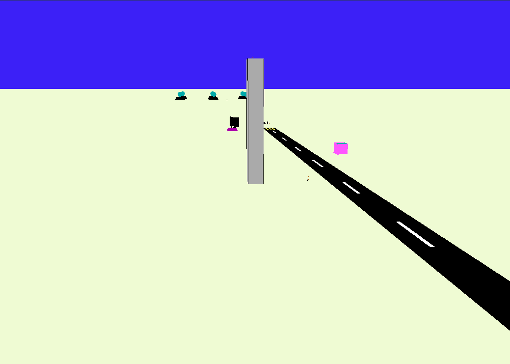
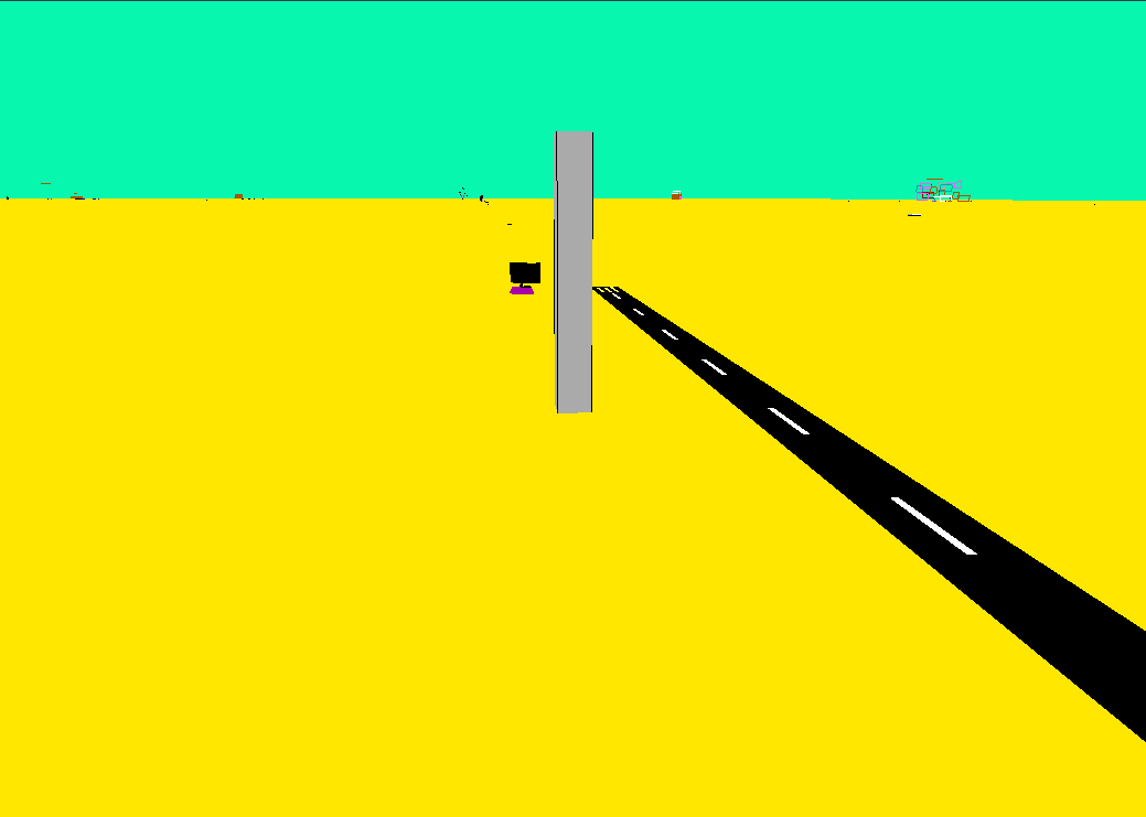
The two views above come from our atlas, using the recovered world colours and models with modern depth testing. The airfield hardware is familiar; the palette supplies much of the change of scene. Select either image to explore its world.
The polygon filler has a special path for colour values above 15. It generates random byte masks, constrained by 0x55, and refreshes the mask on successive scanlines. Selected pixels are written and the gaps retain the background. The resulting broken fill is not alpha blending: there is no calculation of a partly transparent RGB colour.
This path is worth preserving as code rather than describing it as a generic “transparent material”. Its colour setup and masks share register values, and the exact result includes those implementation details. A tidy checkerboard or a modern translucent polygon gives a different effect.
The ground is mostly the horizon
It is easy to imagine an enormous green floor polygon underneath everything. The ordinary background is cheaper than that. Corncob sets a horizon-fill flag, draws its specially prepared horizon object, and fills sky and ground on the appropriate sides. Pitch and bank change the boundary. When the boundary misses a window, the code can fill that window entirely with the correct side.
Objects supply the runway, buildings and alien installations. The background does not need a terrain mesh to stretch to the horizon. There is no textured landscape waiting below the ground dots.
The dots provide motion cues over that otherwise featureless surface. The original keeps a bank of eighty ground points. Replacement positions are generated at ground height in a square around the observer, with a total width of 64 times observer height. A point that remains in view stays anchored in the world; points that fail to draw can be regenerated, and a small random refresh adds turnover.
That dependence on altitude is doing useful work: climb higher and the sampling area grows. It also produces behaviour we noticed while making Redux screenshots. Points can accumulate where the view keeps them alive, and an expanded renderer needs to reconsider their distribution, range and pixel size together. Merely asking for more of the old dots does not guarantee an even-looking field.
Stars use another bank of points, generated at a large fixed height. They are not painted on a skybox texture. The sun is a tiny model using overlapping discs, with its size, angle and colour supplied by the environment. Some earlier versions even give it a face. A skyline containing a smiling sun and a furious little ground crew member is still made from the same few drawing operations.
A cockpit made to survive redrawing
The cockpit surround starts as a compressed one-bit image. The instruments add moving marks over it. The raw image includes a diagonal across the viewing area; we initially exposed that line in extraction. The running game overwrites the view with scenery, so it does not normally remain visible there.
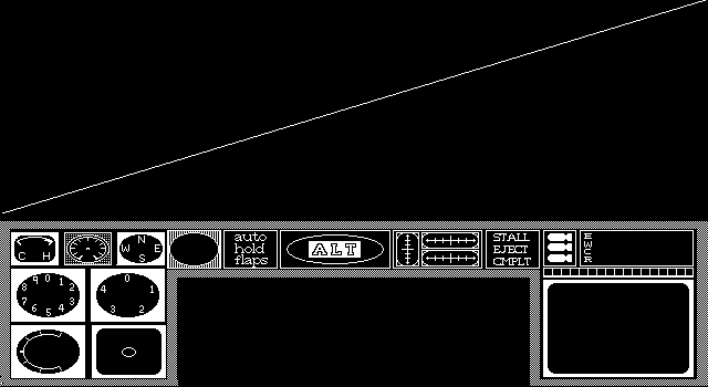
The planar layout gives the instrument code a useful separation. Gauge marks can be written into the high colour bit while preserving the lower three bits of the cockpit image. Setting or clearing that bit changes a pixel’s colour without destroying the underlying artwork. The implementation also spreads updates for several instruments over a fourteen-frame schedule, accounting for the alternating display pages. Not every needle needs the same amount of work on every frame.
Text takes several routes. Menu and tower text uses the normal BIOS lettering. Flight messages explicitly select the BIOS 8 × 14 font. The cockpit labels and help pages are already pixels in their images. The medal characters are the small custom replacement set used by the text interface. There is no hidden general-purpose font engine holding the instrument panel together.
The rear display is not a mirror
The rear window uses the same scene geometry and primitive paths, with a smaller viewport and focal lengths of 150 and 100. For ordinary geometry the XVECT helper negates the forward and sideways coordinates and keeps height. That turns the camera around by 180 degrees.
So an object behind the left wing appears on the right of the rear display, as it would if you turned around to look at it. We had to check the original source to settle this: it really is a backwards camera. Redux now deliberately reflects the display to behave as a mirror; the faithful reconstruction retains the original orientation.
Showing a finished page
The engine alternates two video-memory pages. While the display scans one page, drawing goes to the other. FLIPAGE changes the display start address and switches the drawing offset for the next frame. It does not copy a complete colour image through the CPU to present it.
There is a further hardware shortcut hiding here. Screen shake can alter the displayed start address, shifting the scanned image without transforming the entire world again. The source contains a refresh-wait helper, but the call beside the page flip is commented out: double buffering alone should not be mistaken for a promise of synchronisation to every vertical retrace.
Why the rough edges matter
Corncob’s graphics are simple enough to understand by following a handful of routines, but their behaviour is shared between model data, integer maths, drawing order and the video controller. A head is the wrong size if we misunderstand one word. A windscreen disappears if we simplify a drawing list. A circle changes shape if we forget what the original display did to its pixels.
That is also what makes the renderer satisfying to take apart. The choices are visible. The plain ground explains the need for dots. The absence of a depth buffer explains the care spent on model lists and the special runway pass. The memory layout explains why a shallow line becomes a collection of byte-friendly runs. The round wheels explain why the engine has a whole disc drawer beside its polygon code.
For our faithful reconstruction, those are behaviours to understand and retain. For Redux, they tell us where a deliberate change belongs: depth testing for the tower door, a different ground-detail distribution, square-pixel projection, a mirror that actually mirrors. We can make those choices without accidentally attributing our new renderer’s behaviour to the old game.
The gallery and world atlas are good places to keep pulling at the thread. Look at the crew from the side. Switch an aircraft to its far model. Find the suspended airstrip. There is usually less geometry than you expected, and rather more intent in its arrangement.
Code and evidence
This article follows our own inspection of the original data and routines. The preserved source is an Initial Import snapshot, before later assembler-compatibility edits; it contains experiments as well as shipped paths. Retail 3.42 executable checks resolve the distinction where it matters.
- Original renderer, F3DVEC.ASM: projection, clipping, model dispatch, octant selection, distance evaluation, sorting, span filling, discs and page flipping.
- Original main loop, 3.ASM: horizon, ground points, object traversal and graphics setup. KLINE.ASM contains the shallow-line path; INST.ASM contains the instruments.
- Our readable C++ translations: fixed-point maths, scene drawing, raster routines, and instrument updates. These are reconstruction code, not the original source.
- Extracted resources and format notes, and the complete research browser.
- Article evidence and illustration provenance, including the limits of the interactive examples.
For a more elaborate engine from a couple of years later, our TFX graphics article follows model programs, terrain, textures and cockpit displays through another software renderer.
The picture is only half of the flight. Our flight-physics article follows the controls, lift, engine power and landing-gear logic, with measurements from the original executable.